m_realTimePhys | LMBrown Portfolio

Predicting Physical Motion

Design objectives:

In order to get more accurate control of autonomous navigation and smooth acceleration and deceleration for my FTC robotics software Cuttlefish, I set out to model the behavior of the motor drivers to predict their physical characteristics. In order to do this, I modeled the motor system as a circuit.

Simulation and modeling of electrical systems

First I modeled the motor as a circuit. When a current is applied to a motor, the shaft of the motor experiences a force which causes it to accelerate. As the speed of the motor increases, the voltage across the motor also increases due to the motor acting as a generator. This is known as back-emf. This means that mathematically, the derivative of the voltage across the motor is proportional to the current.

dV/dt =i

This is the same behavior as is seen in the component known as the capacitor. Capacitors experience an increase in voltage due to the accumulation of charge between two plates, while motors experience an increase in voltage due to the increase in rotational velocity of a mass, but the end result is the same.

Due to the fact that motors contain what are essentially electromagnets, motors also have significant series inductance and resistance which can be modeled as a series inductor and resistor respectively.

The motor driver consists of an MOSFET H-bridge, but since we only need to model the behavior in one direction it can instead be modeled as a switch and a diode..

This switch is turned on and off at a fixed frequency with a duty cycle determined by the motor power. This is known as pulse width modulation or PWM. The diode acts as a freewheeling diode, allowing current to continue flowing, even when the switch is open. This means that the overall circuit is equivalent to a buck converter which is a type of DC-DC converter, where in this case, the capacitor is the motor, and the load is the friction on the motor (force is current draw in this context). This is easy to model some of the time. If we assume that the capacitance is big enough to be effectively infinite over one PWM cycle, and that there is always current going through the inductor, then the average DC voltage across the inductor and resistor is equal to PVS - VM where P is motor power, Vs is the supply voltage, and VM is the motor back EMF. Since this is a DC, it will be ignored by the inductor meaning that the current is entirely determined by the resistor (ohm’s law): i = (PVS - VM)/r. However, it is not always this simple. During deceleration, the back EMF of the motor will be less than the average PWM voltage meaning that current will stop flowing through the inductor for part of the PWM cycle which makes the math much more complex. This is equivalent to a buck converter operating in discontinuous mode where there is no current through the inductor for part of the period. I originally modeled this with the effect of the ESR included, but I later realized that the effect of the ESR is small enough to be omitted as the ESR is on the order of 1-2ohm and the discontinuous mode current is less that 500ma meaning that the total effect amounts to less than a volt. Omitting the ESR makes the math much simpler.

These are some of the equations I got by modeling the system as a differential equation and then solving the differential equation. This version was not ideal due to the use of substitution, as much of the complexity was hidden until the end.

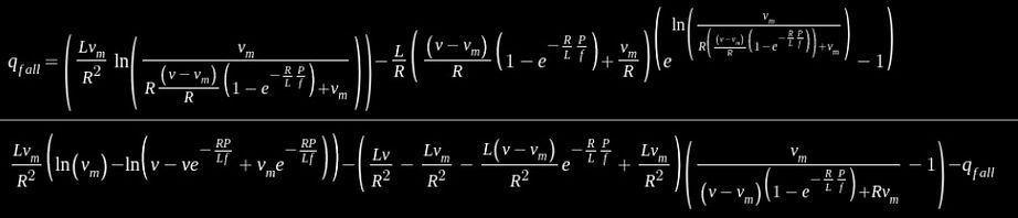
And an improved version after changing the approach to solving the problem.

Simpler derivation

During the on part of the period, the current starts as zero and then rises at a rate proportional to the voltage across the inductor which is (VS - Vm) .

di/dt = (VS - Vm)/L

ion = (VS - Vm)trise/L

t at the end of the on period is equal to the length of the total period time the duty cycle.

trise = p/f

During the off part of the period, the current falls at a rate proportional to the motor back emf until current reaches 0.

di/dt = -Vm/L

i = ion - tVm/L

ion - tfall Vm/L = 0

tfall Vm/L = ion

tfall = Lion / Vm

ton = trise + tfall

The mean current while current is flowing is equal to

ion / 2 and current flows for (ton / f) of the period meaning that:

i = (ton /(1/f)) * ion / 2

Substituting in all of the relevant variables

tfall = (VS / Vm - 1) (p/f)

ton = (VS / Vm - 1) (p/f) + (p/f) = (VS / Vm)(p/f)

ion = (VS - Vm)trise/L

Finding power from current:

Now that we can do motor control by current, we need to calculate control by force. Force should be directly proportional to current. The goBILDA website provides the stall current and stall force of their motors, so this is what we will use as our reference values.

T = i * Tstall / istall

i = Tistall / Tstall

We can now drive motors by force allowing us to do true physics based motion control with friction and mass coefficients, and control velocity without the need for PID or feedforward time based algorithms.

Control by Force

The first step of the navigation algorithm I developed is control by force. I control the robot by telling it how much force to apply to the ground, rather than by how much power. This allows me to achieve smooth motion by setting the maximum force, and improves movement and software characteristics in a variety of ways. First I must determine how much force to apply to the wheels. To do this I modeled mecanum wheels (1) interaction with the ground. Assuming the wheel isn't slipping, and the wheel has negligible mass, the force exerted by the motor on the edge of the wheel must match the force exerted on the wheel by the floor. The force exerted by the wheel is entirely in the Y direction (forward) and is labeled FM. However, the force exerted by the floor on the mecanum wheel must be perpendicular to the rollers, because there is no traction in the direction parallel to the rollers, meaning the force due to traction with the floor FT must be diagonal to the wheel, at an angle of 45 degrees (roller angle).

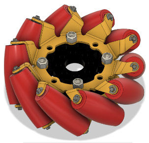
(1) mecanum roller wheel

This is surprising because diagonal force of the wheels is greater than torque being applied by the motor. This makes sense, because when moving forward there are forces canceling inwards, yet the force experienced forward is the same as with normal wheels. Since the force vectors of the wheels are known, the force in chassis space can be converted to wheel space using a linear transformation with the basis vectors in robot space being of: X, Y, R, and G. G stands for “Grind” and is the vector that corresponds to driving the wheels against each other providing no net force. Grind is always set to 0.

Since I can set motor torque based on the speed of the motor, in order to control the chassis using force, I need to determine the speed of all of the chassis motors. To do this I model how mecanum wheels work. By rotating a single mecanum wheel, it is possible for it to move forward like a normal wheel. After rolling it forward, without changing the rotation, you can move it diagonally in the axis of the rollers. Since these two actions are independent, you can reach any location on the diagonal line by rotating the same amount forward. This means that if Dy is the forward displacement after rotating the wheel without sliding, you can get to any point (Dy, 0 ) + vt where v is the vector of the rollers, and t is any real number. If the rollers point such that the wheel can slide forward and to the right, or backward and to the left, then v = (1,1). Dy can be calculated as the number of radians the wheel has rotated ω, times the radius of the wheel r. This means that if v = (1,1) then (rω+t,t).

Written differently: x = rω +t, y = t

Since θ and t are unknown, and x and y are known, the system of equations is determined and can be solved. The result in the case that v = (1,1) is that θ = (x - y) / r. This is surprising because we expect that the combination of x and y would use the Pythagorean theorem, but doing that yields an incorrect result. This process can be repeated for the other diagonal vector (-1,1) to get the equation θ = (x + y) / r. X and y are equal to the x and y displacement of the robot plus the perpendicular of the vector describing the position of the wheel relative to the center of the robot times the rotation in radians.

VXYFrontRightWheel = VXYRobot + PWheel⊥VθRobot

ωFrontRightWheel = (VXYFrontRightWheel.x - VXYFrontRightWheel.y) / r

This can be repeated for all wheels. Once the rotational velocity of the wheels has been calculated it can be used to set the motor torque as described above.

Friction Compensation and Velocity Control

One of the advantages of control by force is it allows for accurate friction compensation. The friction that the robot is experiencing can be calculated and then added to the force, resulting in friction being negated and the robot being placed in what we call “enhanced slippery mode”. When the robot is in enhanced slippery mode, it acts as though it is not experiencing friction and can roll freely across the field when pushed. I can then tune the friction and mass coefficients independently for each wheel with real-time feedback. This is advantageous because it allows for control by velocity with very little steady state error, thereby improving control characteristics. Essentially, I gain all the advantages of open-loop control, with the stability and predictability of closed-loop control.

Additionally, this allows our robot to accelerate and decelerate at the maximum possible value without losing traction, lifting, or spinning out. I have also added a defensive hold position mode for drivers that matches any external force applied. This allows our robot to hold it’s position while other robots attempting to push us spin their wheels.

With friction compensation and control by force, control by velocity can be achieved by simply using proportional controller.